Multiple forms of dynamic representation

Abstract

The terms dynamic representation and animation are often used as if they are synonymous, but in this paper we argue that there are multiple ways to represent phenomena that change over time. Time-persistent representations show a range of values over time. Time-implicit representations also show a range of values but not the specific times when the values occur. Time-singular representations show only a single point of time. In this paper, we examine the use of dynamic representations in instructional simulations. We argue that the three types of dynamic representations have distinct advantages compared to static representations. We also suggest there are specific cognitive tasks associated with their use. Furthermore, dynamic representations of different form are often displayed simultaneously. We conclude that to understand learning with multiple dynamic representations, it is crucial to consider the way in which time is displayed.

Multiple Representations of Time

Dynamic representations display processes that change with respect to time. For example, they may show blood pumping around the body, the flux of high and low pressure areas in a weather map, the developing results of a computer program running (algorithm animation) or the movements in physical systems such as series of pulleys. Animation is normally considered the prototypical dynamic representation and is defined as a “series of frames so each frame appears as an alternation of the previous one” (e.g. ). Typically, each frame exists only transiently to be replaced by subsequent frames, i.e. the dimension used to represent time in the representation is time. refers to this aspect of animation (and other representations such as video and speech) as evanescence, in contrast to still, persistent media such as static pictures or text.

The research on the effectiveness of animation for increasing learners’ motivation normally reports positive effects (e.g. ). However, research addressing whether animation aids learners’ understanding of dynamic phenomena has produced positive results ( ; ), negative results (; ) or neutral results (; ). This is not surprising as a single type of representation is rarely maximally effective for all purposes, but rather particular representations facilitate performance on certain tasks ().

Nevertheless, there are a number of reasons why research on animation effectiveness has produced such mixed results. A wide range of factors such as outcome measures, individual differences in participants and research environment have been varied, making consistent results less likely (). Nor has only a single type of animation been investigated. identifies three types of change events used in animations: transformations, in which the properties of objects such as size, shape and colour alter; translation, in which objects move from one location to another; and transitions, in which objects disappear or appear. Learners may focus on more obvious perceptual events rather than on those that are of most conceptual interest – for example, found that novices extracting information from a dynamic weather map focused on less important translations rather than the more important but perceptually subtle transformations.

There are a number of reasons why animations may place increased demands on learners. analyses animations (as simple as a guide to constructing ‘flat-pack’ furniture) from a perspective that emphasises the semantics and processing requirements of making inferences from representations (see for details of the approach). Firstly, he argues that as the information in animations is presented transiently, relevant previous states must be held in memory if they are to be integrated with new knowledge. Secondly, animations cannot be ambiguous with respect to time and, as a consequence, they force activities to be shown in a particular sequence. Consequently, when what is represented is not fully determined with respect to time, animations may employ tricks (such as showing activities happening in parallel like nails being hammered into a table top simultaneously) or place activities in a particular order where in fact order is irrelevant (and in text could easily be expressed as “now hammer in all four nails”). Thirdly, unlike a static diagram, animations that are not user-controllable do not permit learners to re-access previous states or vary the speed at which information is presented.

However, not all work identifies transiently presented information as a necessary aspect of animation. proposes that persistence is, in fact, a dimension of animation (i.e. representations can range from those that only define the current state of the information to those that contain a history of each change in information). Hence, some of the difficulties associated with processing animations should not apply to dynamic representations that are persistent. In particular, these representations should not lead to the memory loads associated with integrating transient forms of representations. Additionally, learners can inspect previous states at will in persistent representations. However, persistence may cause representations to be very complex if all prior states have to be explicitly represented.

In this paper we shall examine how persistence influences both the informational and computational properties of dynamic representation. Furthermore, dynamic representations are almost never presented in isolation but are usually combined with textual description of the situations, pictures or other forms of representation. Hence, we focus on the impact on learners of combining representations with different dynamic form. We will illustrate this argument with a type of learning environment that almost invariably employs multiple dynamic representations – instructional simulation. We begin by describing the properties of simulations and provide an example to use as a case study throughout the rest of the paper.

Instructional Simulations

Instructional simulations such as SimQuest () or Stella () are domain independent environments that contain an executable model of a system whose results are presented to learners. They allow learners to construct their own knowledge by interacting with an environment, conducting experiments and by observing the effects of these experiments. As a consequence, it is hoped that learners acquire deep, flexible, and transferable knowledge. Simulations overcome one of the limitations of natural systems by allowing representation of processes and quantities that are usually invisible in nature (e.g. energy, vectors, equilibrium states, etc.). They almost always provide multiple external representations of the simulated model. For example, a simulation of a harmonic oscillator (e.g. ) can present the motion of the system by a basic animation of a body’s movement and also by graphically representing this motion in time-series graphs or as phase-plots (for definitions see below). Moreover, both graphs and animation can be presented simultaneously, allowing observation of the interrelation between the two representations.

In this paper, we will draw all examples from a simulation of population dynamics (see ). Population dynamics is the branch of biology that attempts to discover the rules that govern how populations of living organisms grow, decline or oscillate. It describes such features as a species birth/death rate, the maximum number of individuals that can be supported in a population, the rate that predators capture prey and how availability of prey influences the number of predators that can be supported. The relationship between these features is given by fairly complex mathematical expressions. For example, a simplified statement of the relationship between number of predators and prey is given by Lotka-Volterra equations such as dN/dt = r N(1-N/K) – alpha N P, (where r = prey fertility, N = population density of prey, P = population density of predators, K = carrying capacity of the environment and alpha = the number of prey killed by a predator per unit time). However, as may be immediately apparent to the reader, this is a dense expression which learners can find difficult to interpret.

To help learners understand such complex relationships, textbooks typically provide a number of forms of representations such as time-series graphs (e.g. the population density of number of prey and predators on the Y axis with time of the X axis), Ln(X) graphs (e.g. the Y- Axis represents the natural log of population density with time on the X axis), phase-plots (e.g. the number of prey on the X-Axis and number of predators on the Y-Axis), tables of values, histograms, piecharts, text that provides definitions of terms and pictures of the animals described. The advent of instructional simulations expands this representational repertoire in two ways: firstly, by changing static representations into their dynamic equivalents (e.g. a time-series graph can incrementally adjust as the simulation runs or as learners interact with it) and secondly, by allowing new forms of representation such as video or animation.

Dynamic Representations in Instructional Simulations

There are many ways of classifying representations. Commonly representations are discussed in terms of features such as their modality (text or graphics), abstraction (e.g. iconic or symbolic), sensory channel (auditory or visual), dimensionality (i.e. 2 d or 3d) or dynamism (static or dynamic). In this paper, we argue that to classify representations merely as either static or dynamic is to categorise at the wrong level of granularity. Instead, we propose that in addition to static representations, there are three types of dynamic representation. We contend that each has distinct informational and computational properties.

Time-persistent representations

The first type of dynamic representation is one we call a time-persistent (T-P) representation. It expresses the relation between at least one variable and time by displaying both (i) the current value and (ii) any other ones that have been computed. Typical examples in this domain include a graph of the population density of predators and prey against time (time-series graph) or a table where each row contains the number of prey killed (e.g. Figure 1). In many ways, this type of representation is very similar to its static equivalent. Often the only difference between this representation when presented in a textbook or in a simulation is that the dynamic representation displays data incrementally rather than presenting the whole data set from the start. Taking a timeseries graph and making it dynamic does not add any new information, although it may make certain features of that information more salient. This is not the case for the other forms of dynamic representation discussed later. For example, if the learner stops the simulation running, it is still possible to determine how fast populations are growing or declining by examining the scale of the representation and previous values of the variables. Therefore, for any dimension of information that a T-P representation displays, it provides the learner with the most amount of information. The finer the granularity of the representation of time the greater this information (e.g. contrast the categorical table with values presented only once every 5 steps of the simulation (Figure 1a) versus a continuous time-series graph (Figure 1b)).

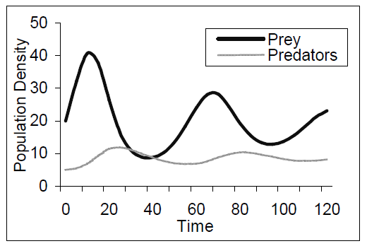
Figure 1

Time Persistent Representations: Predator Prey Population Density (a) Table, (b) Time-Series Graph

Figure 1

Time Persistent Representations: Predator Prey Population Density (a) Table, (b) Time-Series Graph

Time-implicit representations

The second type of representation is time-implicit (T-I), which show a range of values but not the time when these values occurred (once static). The most common example in population dynamics is a phase-plot (or phase space graph) where the X-axis encodes the number of prey and the Y-axis the number of predators, and time is the parameterising variable along the plot line (see Figure 2, 2a is generated from the same information as Figure 1).

Like T-P representations, T-I representations show the relation between variables over a period of time. Unlike the T-P representations, however, the time-scale of this information is only perceivable when presented dynamically. For example, Figure 2a, shows that when the number of prey was 41, the numbers of predators was 7, but although we know this happens in the past, there is no way to determine what point in time this occurred. The rate of change of the values being graphed is only visible when the simulation is running and the representation dynamically adjusting. Consequently, when a simulation is stopped learners must invoke internal representations to compare current values to a particular previous state to answer questions about the timescale of growth. Thus, this representation has different information when presented dynamically than when presented statically. For example, in static Figure 2a, there is now no way of determining how long it took for prey numbers to increase from 20 to 40. Similarly, Figure 2b shows a limit cycle and so it is impossible to know how many times this cycle has occurred when presented statically, whereas this information would be obvious in a time-series graph. As a result, these representations contain less information that T-P, i.e. it is possible to derive a T-I representation from a T-P representation but not vice versa.

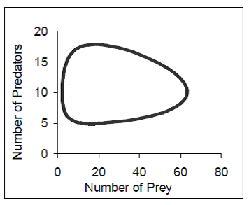
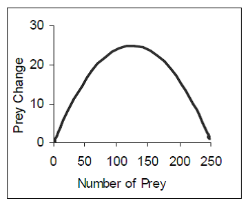
Figure 2

Time Implicit representations: (a, b) Predator Prey Population Density Phase-plots , (c) Population Change v Population Density Phase-plot

Figure 2

Time Implicit representations: (a, b) Predator Prey Population Density Phase-plots , (c) Population Change v Population Density Phase-plot

Time-singular representations

The third type of representation, time-singular (T-S), displays one or more variables at a single instant of time. We consider this to be the classical case of animation as this type of representation is evanescent. Examples of T-S representations that are useful for understanding population dynamics include a pie-chart of the relative proportions of prey and predator density at a particular instant of time, a picture of caterpillar which adds a new segment to its body for every 100 new bugs born or a histogram of the values of population density, etc. Of course, in many cases this is not an intrinsic property of the representation. A histogram could be designed such that a new bar represents a new point in time. In that case, it would have been a time-persistent representation.

Figure 3

Time Singular representations: Population density (a) Dynamic Text, (b) Pie Chart, (c) Concrete Animation.

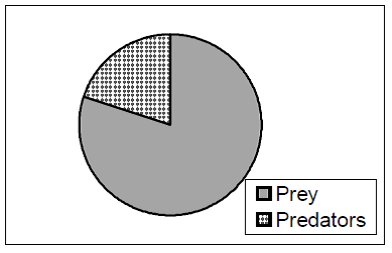
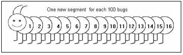
Figure 3

Time Singular representations: Population density (a) Dynamic Text, (b) Pie Chart, (c) Concrete Animation.

As T-S representations display only one state of the system at a time, they contain less information per dimension compared to T-P and T-I representations. As a result, they are often used when the information to be conveyed is highly complex and involves many interacting elements (such as weather systems or blood pumping through the body). But as a consequence, when a simulation is stopped the external representation contains only limited information, placing higher demands on internal processing. For example, to compare current values to previous ones, learners must hold previous states in memory to integrate them with new information and such activities are known to place heavy loads on working memory. T-S representations that don’t allow for learner control (e.g. scrolling forward and backward) are therefore likely to prove very demanding. Learners must also internally represent the rate of change of the values to determine the velocity of change.

Static representations

Finally, dynamic simulations often include static representations. Examples of these include a picture, a written text defining terms or the Lotka-Volterra equations (Figure 4). These representations allow learners to scan over them at their own initiative, whether the simulation is running or still. In this sense, they are similar to T-P representations. They are only intended to show a single state of the world, like T-S representations, but unlike T-S representations they never change. When included in dynamic simulations, they place different demands upon learners than when presented in static media. For example, for system designers, it is easy to know when a representation is not intended to change with time. However, learners may have to inspect static representation at some length to rule out the possibility that it is a single snapshot of a potentially varying T-S representation.

Figure 4

Static representations: (a) Definition of Terms, (b) Static Graphic (c) Equation

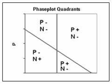
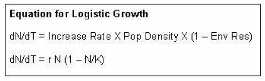
Figure 4

Static representations: (a) Definition of Terms, (b) Static Graphic (c) Equation

Analysing Learning withMultiple Dynamic Representations

We have previously argued that most instructional simulations (and indeed almost all learning environments) involve multiple representations. Multiple representations can offer unique benefits when people are learning complex new ideas (; ) and are often a characteristic of expertise and expert communication (e.g. ; ) but unfortunately many studies have found that these benefits are not always easily achieved (; ; ). To identify the reasons for these mixed results, we developed the DeFT (Design, Functions, Tasks) framework for learning with multiple representations (e.g. ). It proposes that to understand how multiple representations influence learning, three fundamental aspects of learning should be considered: the design parameters that are unique to learning with more than one representation; the different pedagogical functions that multiple representations can play; and the cognitive tasks that must be undertaken by a learner when interacting with multiple representations.

In this paper, we use the functional taxonomy of multiple representations to argue that dynamic representations can play many different roles in learning. proposed that the functions of multiple representations fall into three broad classes. Firstly, multiple representations can support learning by allowing for complementary computational processes or information. Secondly, multiple representations can be used so that one representation constrains interpretations of another. Thirdly, multiple representations can support the construction of deeper understanding when learners abstract over representations to identify what are shared invariant features of a domain and what are properties of individual representations.

Complementary Functions of Dynamic Representations

When multiple representations complement each other they do so because they differ either in the information each expresses or in the processes each supports. By combining representations that differ in these ways, it is hoped that learners will benefit from the advantages of each of the individual representations.

Multiple representations provide complementary information when a single representation would be insufficient to carry all the information about the domain. Multiple representations provide varying computational processes when they provide learners with the opportunities to draw alternative inferences about the domain (e.g. , ; ). This is one of the most common reasons to use multiple representations and can be advantageous as different representations support different tasks (e.g. ), alternative strategies (e.g. ) and individual differences (e.g. ).

By definition, time-persistent, time-implicit and time-singular representations express different information. This can be demonstrated using population density of predators and prey (P & N) as an illustration. The T-S representation (Figure 3a) show the current value of N and P, the T-I representations show the relation between N & P since the simulation starting running but without information about when N and P were at these values (Figure 2a,b) and the T-P representations show all values of P and N that are available since the simulation began running (Figure 1). Thus, system designers can exploit these different informational properties of dynamic representations. They can provide T-P and T-I representations to encourage learners to consider the range of values and their relationship to each other time. T-S representations can provide a simple display of current value and are particularly useful if learners are allowed to manipulate information in the simulation.

The different types of dynamic representations also have different computational properties. Time-persistent representations do not suffer from the problems of transience associated with animation and so for many tasks working with this type of representation will be easier for learners. Furthermore, learners have considerable control over this form of dynamic representation, as it is easy for them to inspect previous states when they chose. To integrate information about past and present events, a learner working with a T-P representation can simply compare values by reading the external representation, so off-loading computation (e.g. ). In contrast, in evanescent T-S representations this can only be done by invoking either the memory of previous states or by performing some inferential step. As a result, we would expect T-P representations will help learners to perform tasks that involve both current and previous values by reducing the memory requirements of holding previous states in memory to integrate with current ones. Time-persistent representations are ideal for showing relationship between current and past values of a variable. They allow learners to compare two discrete points easily (e.g. in a table) or to inspect the overall pattern (time-series graph). They also can facilitate prediction of future values particularly when there is a simple and obvious perceptual cue (e.g. a straight line of a Ln(N) v Time graph for exponential growth or the “s” shape of logistic growth).

Time-implicit representations are excellent for determining the relationship between two dimensions of information at a particular point in time. Previous research has shown that people find the specific value of one variable at a given value of another variable in less time when presented with a phase-plot rather than that a time-series graph even when they are more familiar with timeseries graphs (e.g. ). They can allow learners to quickly determine the type of relationship between predators and prey and help learners predict future values but not when these values will occur. For example, the phase-plot in Figure 2 facilitates estimation of where the stability point is (roughly when N = 20 and P = 8) but not when it will occur. Figure 2b shows that the populations will continue to oscillate without ever reaching a steady state as the graph shows a limit cycle. Figure 2c shows that the maximum rate of change for a population growing logistically occurs when population density is at the midpoint of carrying capacity.

T-S representations provide a quick overview of the current value of the simulation. They facilitate comparison between two or more dimensions of information when time is not a factor (e.g. computing increase rate by subtracting death rate from birth rate). T-S representations are concise and take up little screen space. For example, there is little point including a table of values of birth rate, death rate, etc when for all 300 steps of the simulation the values stay the same. It is also an ideal form of representation when the information to be displayed includes static values (such as the carrying capacity of a population) and dynamic values (such as population density).

This may be one of the most common reasons to include multiple types of dynamic representations. To fully understand such complex phenomena many different types of inference are required - some quantitative with respect to time and some qualitative. The flexibility afforded to the learner by providing multiple dynamic representations mean they (or the system designer) can chose which representation best support the current educational objective. Of course for each representation added to the system, learners must understand how to interpret its format and operators. T-S representations generally have simple format and operators. T-P representations are more complex. However, most learners will be familiar with their static equivalents and we have argued that T-P representations are much closer to their static equivalents than other forms of dynamic representation. However, although T-I representations share the same format as T-P representations such as timeseries graphs, even simple changes in form affects learners’ understanding of line-graphs (e.g. ). So although learners should be able to apply previously learnt operators such as determining maxima and gradients, they may have difficulty determining what these features mean in the T-I representations. This can lead to misconceptions such as assuming that greater distance on the X-axis means greater time. Consequently, learners may need additional help in understanding this type of representation (see Constraining Functions).

Constraining Functions of Dynamic Representations

A second use of multiple representations is to help learners develop a better understanding of a domain by using one representation to constrain their interpretation of a second representation. For this use of dynamic representations and, in contrast to complementary functions of dynamic representations, it is crucial that learners understand the relation between the representations.

The first way that constraints tend to be achieved is by employing a familiar representation to support the interpretation of a less familiar one. For example, familiar concrete representations such as simple animations are often employed in simulations to support interpretation of complex and unfamiliar representations such as graphs. Simpler T-S representations (e.g. the dynamic values in Figure 3a) may help learners interpret more complex T-P and T-I representations.

The second way that constraints can be achieved is by taking advantages of inherent properties of representations. For example, graphical representations are generally more specific than textual representations (e.g. ). So, when textual and graphical representations are presented together, interpretation of the textual (ambiguous) representation may be constrained by the graphical (specific) representation. Consequently, a representation can aid in interpreting another is when its inherent properties make something explicit that is only implicit in the other representation. A classic example is the way that the timescale is explicit in T-P representations but only implicit in other representations. For example, most learners are considerably less familiar with the way that time is given by the curve in phase-plots rather than on the X-axis as in time-series graphs. Hence, presenting both representations simultaneously can provide learners with the tools to understand the phase-plot, if they can see how it relates to the timeseries graph.

Constructing Functions of Dynamic Representations

Multiple representations can support the construction of deeper understanding when learners integrate information from multiple representations to achieve insight it would be difficult to achieve with only a single representation. ‘Deeper understanding’ is considered as abstraction, extension or relational understanding. Abstraction is the process by which learners create mental entities that serve as the basis for new procedures and concepts at a higher level of organization. For example, argues that perceptual variability (the same concepts represented in varying ways) provides learners with the opportunities for building such abstractions. Extension is the process by which a learner extends knowledge from a known to an unknown to representation, but without fundamentally reorganizing the nature of that knowledge. Relational understanding is considered to be the process by which two known representations are associated, without reorganization of knowledge. The differences between these functions of multiple representations are quite subtle and all may be present at some stage in the life cycle of encouraging deeper understanding with a multirepresentational environment.

The many different forms of dynamic representation support learners coming to understand population biology because of the complementary and constraining functions that they serve. However, it may be the case that if learners can come to understand the relation between the representations, they come to understand the domain more thoroughly. For example, the combination of concrete representations of biology entities as well as abstract representations of mathematical expressions may encourage learners to see population biology as one instance of a dynamical system. There is considerable perceptual variability in how the concepts are represented. The possibility for representational extension also exists. As learners become more familiar with phase-plots of population dynamic by relating them to more familiar representations, they may subsequently be better placed to understand phase graphs in different domains (such as plotting the motion of a pendulum as phase-plot of velocity and position). They may also understand complex multidimensional phase space graphs more easily (e.g. in the classic Lorenz's model of chaos in weather systems) and be able to extend the operators they have learnt to use with phase-plots of population dynamics (e.g. finding attractors, repellers and saddle points).

However, for multiple dynamic representations to support deeper understanding learners must relate the representations to each other. This is likely to cause learners particular problems as previous research on learning with multiple representations has indicated that translation can be the most difficult aspect of learning with multiple representations (e.g. ; ) and furthermore, we know that learner can have difficulties in recognising the relationship between an animation and its static equivalent (e.g. ). Consequently, learners may need particular support in this aspect of learning with dynamic representations.

Conclusions

In this paper, we have argued that it is worthwhile considering the way that time is used in dynamic representations. Although by far the most commonly researched form of dynamic representation is the animation, simulation environments use a variety of representations that have substantially different forms to that of animation. We propose that dynamic representations can take three forms, time-persistent which explicitly shows a range of values using a spatial dimension to indicate time, time-implicit which also show a range of values but not when those values occur and time-singular which only show one value of a variable at a time. We proposed that T-S representations differ the most from their static equivalents, T-I differ somewhat and T-P representations do not differ significantly when presented dynamically.

In the majority of simulation environments learners will often be presented with these different forms of representations simultaneously. We have maintained that the different informational and computational properties of the different dynamic forms of representations means that by combining representations, learners will be able to benefit from the complementary, constraining (and potentially constructing) functions of these different types of representations. However, it will increase the cognitive tasks that learners must complete in order to successfully learn about the concepts and representations under study. For example, Lowe’s research on dynamic (T-S) weather maps (e.g. ) suggests that learners focus on perceptually compelling rather than thematically relevant information. If these features could be extracted from the model and presented in the form of T-P representation, it would be interest to discover whether this would help learners focus on important concepts by presenting them in ways that decrease cognitive load or whether it would hinder learners because of the problems associated with relating representations of different forms.

Little research has directly compared learning with these different forms of dynamic representations. We found some evidence that learners are sensitive to these factors when analysing learning with an instructional simulation (). For example, students interacted exclusively with T-P or T-I representations even when choosing to display significant numbers of T-S representations. No other way of classifying representations (e.g. modality, abstraction, complexity) predicted this relationship. However, we have only just begun to examine of the impact of these different forms of representations in simulations. More fine-grained studies are needed to explore if learners are making strategic decisions about what sorts of representations best support their developing understanding of population dynamics. If we are to effectively support learners as they come to understand the relationship between different forms of dynamic representation, more research is needed to examine the processes by which this occurs It is apparent that multi-representational dynamic simulations afford learners new ways of visualising complex domains. Animation is the most extensively studied form of dynamic representation, but we argue that in many cases, using other forms of dynamic representations either by themselves or in tandem with animations may lead to more effective learning. Research to address how to maximise these advantages of different dynamic representations without overwhelming learners with their associated costs should be productive given the increasing use of all forms of dynamic representations in learning environments.

Acknowledgements

References

Notes